Counter-current imbibition in a quasi-one-dimensional porous medium

Problem Description

This benchmark simulates capillary-driven counter-current imbibition in a homogeneous porous medium, following the McWhorter–Sunada problem. Initially, the wetting phase is at its residual saturation. Wetting fluid enters from the left, displacing non-wetting fluid back toward the same boundary. Gravity, sources and total flow are absent, so capillary pressure is the driving force.

Assumptions:

no gravity
immiscible two-phase flow
incompressible phases
homogeneous permeability and constant porosity
isothermal flow
no source terms
zero total flux (counter-current flow)

For each phase \(\alpha \in \{w,n\}\), the mass balance is

\begin{align}\frac{\partial (\phi \rho_\alpha S_\alpha)}{\partial t} + \nabla\cdot(\rho_\alpha \mathbf{v}_\alpha)=0,\end{align}

and Darcy's law gives

\begin{align}\mathbf{v}_\alpha=-K\lambda_\alpha(\nabla p_\alpha-\rho_\alpha\mathbf{g}), \qquad \lambda_\alpha=\frac{k_{r\alpha}}{\mu_\alpha}.\end{align}

With incompressible phases, constant porosity, no gravity, and zero total flux, eliminating the phase pressures and fluxes gives the one-dimensional saturation equation

\begin{align}\phi\frac{\partial S_w}{\partial t} =\frac{\partial}{\partial x}\left(D(S_w)\frac{\partial S_w}{\partial x}\right),\end{align}

where

\begin{align}D(S_w)=-K\frac{\lambda_w(S_w)\lambda_n(S_w)}{\lambda_w(S_w)+\lambda_n(S_w)} \frac{\mathrm{d}p_c}{\mathrm{d}S_w}.\end{align}

Here \(S_w\) denotes the wetting-phase saturation. The model uses the wetting pressure \(p_w\) and non-wetting saturation \(S_n\) as primary variables.

Semi-analytical Reference Solution

The McWhorter–Sunada solution is an integral solution, rather than an explicit elementary formula. The implementation follows method B of Fučík et al. [39].

The solution assumes a semi-infinite domain and similarity in \(\xi=(x-x_{\min})/\sqrt{t}\). Let \(s\) denote wetting saturation, \(s_i=S_{wr}\) the initial saturation, and \(s_0=1-S_{nr}\) the wetting saturation at the left boundary. For the closed right boundary, the total flux parameter is \(R=0\) and method B iterates the integral function

\begin{align}G(s)=\frac{D(s)}{F(s)},\qquad I(s)=\int_s^{s_0}(v-s)G(v)\,\mathrm{d}v,\qquad F(s)=1-\frac{I(s)}{I(s_i)}.\end{align}

The iteration starts with \(G=D\) and updates \(G=D/F\) after each integral evaluation. It stops when the relative change in the integrand falls below Reference.Tolerance. The converged solution gives a monotone similarity profile, which is interpolated at the cell centers. The profile is computed once, while time sets its spatial scale through \(\sqrt{t}\). Piecewise-linear quadrature and cumulative integrals keep the iteration efficient. The regularized Brooks–Corey endpoint limits are included explicitly.

Fučík's method suits this benchmark because it evaluates the McWhorter–Sunada integral solution with the same capillary and relative-permeability laws as the numerical model. The solution is semi-analytical, such that saturation integrals and iteration are computed numerically. With zero total flux, the original integral iteration converges without extra stabilization. Fučík's more general stabilization is useful when total flux is nonzero.

Parameters

Parameter	Symbol	Value	Unit
Permeability	\(K\)	\(1\text{e-}13\)	m²
Porosity	\(\phi\)	\(0.2\)	-
Brooks–Corey uniformity parameter	\(\lambda\)	\(3.0\)	-
Capillary entry pressure	\(p_{c,e}\)	\(8000\)	Pa
Residual wetting saturation	\(S_{wr}\)	\(0.2\)	-
Residual non-wetting saturation	\(S_{nr}\)	\(0.2\)	-
Wetting-phase dynamic viscosity	\(\mu_w\)	\(1\text{e-}3\)	Pa·s
Non-wetting-phase dynamic viscosity	\(\mu_n\)	\(1\text{e-}3\)	Pa·s
Wetting-phase density	\(\rho_w\)	\(1000\)	kg/m³
Non-wetting-phase density	\(\rho_n\)	\(1000\)	kg/m³

Setup

The implementation uses the DuMux fully implicit two-phase model (2p) with TPFA discretization. A two-dimensional Dune::YaspGrid represents the effectively one-dimensional domain

\begin{align}\Omega=[0,2\,\mathrm{m}]\times[0,1\,\mathrm{m}],\end{align}

with one cell in the y-direction. The default run uses 400 cells in the x-direction and ends at \(3\times10^6\) s. The final time is selected so the semi-infinite reference front remains inside the finite computational domain, including on the coarser grids used for comparison.

Initially \(S_w=S_{wr}\) and \(S_n=1-S_{wr}\). The initial wetting pressure is \(p_w=p_{n,\mathrm{inj}}-p_c(S_{wr})\), where \(p_{n,\mathrm{inj}}\) is the prescribed non-wetting injection pressure. At the left boundary, Dirichlet conditions set \(S_w=1-S_{nr}\) and \(p_n=p_{n,\mathrm{inj}}=1e5\text{Pa}\). Because \(p_w\) is the primary pressure, the corresponding boundary value is \(p_w=p_{n,\mathrm{inj}}-p_c(1-S_{nr})\). The top, bottom and right boundaries are no-flow Neumann boundaries. No fluid can leave through the right boundary. During counter-current imbibition, the non-wetting phase flows back toward the left inlet.

Result and Validation

Run the benchmark and generate the comparison plots with:

python3 compile_run_plot.py

The script expects PyVista and Matplotlib for post-processing. It builds and runs the 200- and 400-cell cases and saves these figures in build-cmake/test/porousmediumflow/2p/mcwhortersunada:

mcwhortersunada_lineplot_comparison.png: numerical \(S_w\) profiles on both grids and the Fučík reference
mcwhortersunada_sw.png: wetting-phase saturation field on the 400-cell grid

Line plot

Saturation field

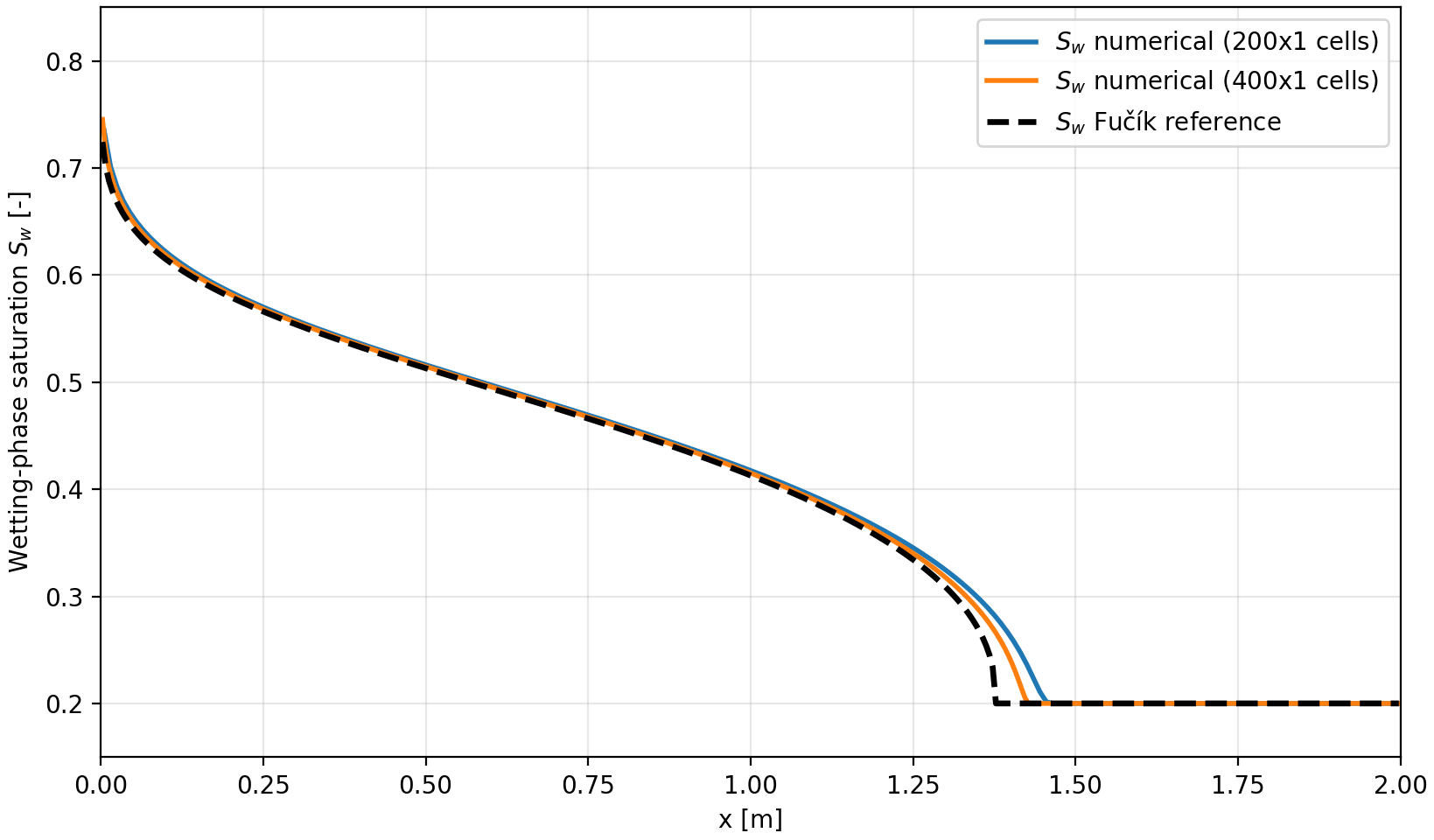
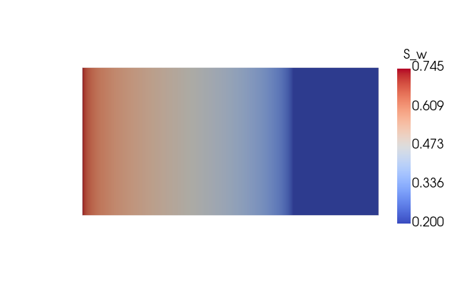
At the end of each run, the test compares imbibed wetting-phase mass, its center of mass measured from the inlet, and the cell-center saturation L1 error with the semi-analytical reference. The mass and L1 errors are normalized by the reference imbibed mass. The residual saturation is subtracted before integration so it does not hide errors in the imbibed plume. Problem.MaxRelError applies the same 4% limit to all three checks.

🛠 Edit above doc on GitLab