 |
version 3.11-dev
|
|
version 3.11-dev
|
Problem Description
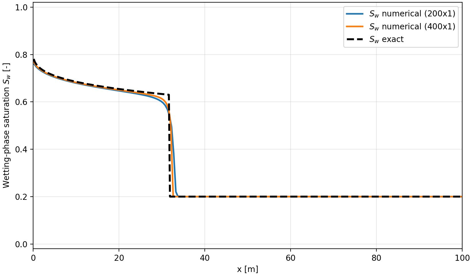
We simulate immiscible two-phase displacement in a quasi-one-dimensional homogeneous porous medium in the classical Buckley-Leverett setting [19]. One phase displaces another phase by viscous forces, while capillary and gravity effects are neglected. The test checks if the numerical scheme captures the hyperbolic transport behavior of the two-phase model at saturation front by comparing to an analytical solution.
Assumptions:
For each phase alpha in \(\{w, n\}\), the mass balance is
\begin{align}\frac{\partial\left(\phi \rho_\alpha S_\alpha\right)}{\partial t} + \nabla\cdot\left(\rho_\alpha \mathbf{v}_\alpha\right) = q_\alpha, \qquad \alpha \in \{w, n\},\end{align}
while the phase flux is given by Darcy's law:
\begin{align}\mathbf{v}_\alpha = -\lambda_\alpha K\left(\nabla p_\alpha - \rho_\alpha \mathbf{g}\right),\end{align}
with phase mobility
\begin{align}\lambda_\alpha = \frac{k_{r\alpha}}{\mu_\alpha}.\end{align}
As described in the assumptions, gravity and capillary effects are neglected, resulting in:
\begin{align}\mathbf{v}_\alpha = -\lambda_\alpha K\nabla p,\end{align}
where \(p = p_n = p_w\) since \(p_n - p_w = p_c(S_w) = 0\).
By treating the phases as incompressible, the porosity as constant and neglecting the source term, the mass balance reduces to:
\begin{align}\phi \frac{\partial S_\alpha}{\partial t} + \nabla\cdot\mathbf{v}_\alpha = 0, \qquad \alpha \in \{w, n\}.\end{align}
Since the saturation constraint
\begin{align}S_w + S_n = 1\end{align}
is employed and the phases share pressure values, it is sufficient to inspect the mass balance equation of one phase, here the wetting phase:
\begin{align}\phi \frac{\partial S_w}{\partial t} + \nabla\cdot\mathbf{v}_w = 0.\end{align}
In 1D, the water fractional flow is defined as
\begin{align} f_w(S_w) = \frac{\mathrm{v}_w}{\mathrm{v}_t} \end{align}
with the total Darcy velocity
\begin{align} \mathrm{v}_t = \mathrm{v}_w + \mathrm{v}_n = -K\left(\lambda_w + \lambda_n\right) \frac{\partial p}{\partial x}.\end{align}
Utilizing the Darcy velocities, the water fractional flow reduces to
\begin{align} f_w(S_w) = \frac{-K \lambda_w \frac{\partial p}{\partial x}}{-K\left(\lambda_w + \lambda_n\right) \frac{\partial p}{\partial x}} = \frac{\lambda_w(S_w)}{\lambda_w(S_w) + \lambda_n(S_w)}.\end{align}
With
\begin{align} \mathrm{v}_w = f_w(S_w) \mathrm{v}_t,\end{align}
the wetting-phase mass balance in 1D can be reformulated to
\begin{align}\phi \frac{\partial S_w}{\partial t} + \frac{\partial}{\partial x}\left( f_w\left(S_w\right) \mathrm{v}_t\right)= 0.\end{align}
Assuming incompressibility the total velocity is constant, resulting in:
\begin{align}\phi \frac{\partial S_w}{\partial t} + \mathrm{v}_t\frac{\partial}{\partial x} f_w(S_w)= \phi \frac{\partial S_w}{\partial t} + \mathrm{v}_t\frac{\text{d} f_w(S_w)}{\text{d} S_w} \frac{\partial S_w}{\partial x} =0,\end{align}
which is the Buckley-Leverett equation in quasi-linear form.
Analytical Reference Solution
The analytical solution follows the standard Buckley-Leverett construction. Characteristic speeds are proportional to the derivative of the fractional flow curve:
\begin{align}x(S_w, t) = \frac{\mathrm{v}_t}{\phi}\frac{\mathrm{d} f_w}{\mathrm{d} S_w} t.\end{align}
The physically admissible shock is selected by the equal-area construction. The implementation samples the saturation interval between \(S_{wr}\) and \(1 - S_{nr}\), computes the fractional-flow derivative numerically, and reconstructs the analytical wetting saturation profile on the cell centers.
Parameters
| Parameter | Symbol | Value | Unit |
|---|---|---|---|
| Permeability | \(K\) | \(1.01936799\text{e-}14\) | m² |
| Porosity | \(\phi\) | \(0.2\) | - |
| Uniformity parameter | \(\lambda\) | \(4.0\) | - |
| Entry pressure | \(p_c\) | \(0\) | Pa |
| Residual wetting-phase saturation | \(S_{wr}\) | \(0.2\) | - |
| Residual non-wetting-phase saturation | \(S_{nr}\) | \(0.2\) | - |
| Constant wetting-phase dynamic viscosity | \(\mu_w\) | \(1\text{e-}3\) | Pa*s |
| Constant non-wetting-phase dynamic viscosity | \(\mu_n\) | \(1\text{e-}3\) | Pa*s |
| Constant wetting-phase density | \(\rho_w\) | \(1000\) | kg/m³ |
| Constant non-wetting-phase density | \(\rho_n\) | \(1000\) | kg/m³ |
Setup
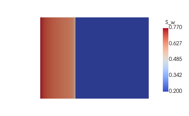
The implementation uses the current DuMux fully implicit finite-volume two-phase model (2p) with TPFA discretization. The computational domain is represented by a two-dimensional Dune::YaspGrid on \(\Omega = [x_\text{min}, x_\text{max}] \times [y_\text{min}, y_\text{max}] = [0, 100\,\mathrm{m}] \times [0, 75\,\mathrm{m}]\), with \(200 \times 1\) grid cells, so the problem is effectively one-dimensional. The wetting phase is initially at residual saturation. At the left boundary, all primary variables are prescribed via Dirichlet conditions, while a constant non-wetting mass outflow is imposed as a Neuman condition at the right boundary. Top and bottom boundaries are no-flow boundaries.
Result
To run the test and produce plots below, execute:
The script expects PyVista and Matplotlib to be available for post-processing.
The script produces two figures in the build-cmake directory:
 3.11-dev
Generated by
3.11-dev
Generated by  1.16.1