Verification of Multi-Stage Time Integration Schemes

Problem Description

DuMux implements a family of one-step multi-stage time integration schemes in Shu-Osher form [78] (see MultiStageMethod). Given the semi-discrete problem

\begin{align}\frac{\partial M(x,t)}{\partial t} - R(x,t) = 0, \end{align}

an \(m\)-stage scheme advances the solution from \(t^n\) to \(t^{n+1}=t^n+\Delta t^n\) via

\begin{align}\sum_{k=0}^{i}\Big[\alpha_{ik}\,M\big(x^{(k)}, t^n+d_k\Delta t^n\big) + \beta_{ik}\,\Delta t^n\, R\big(x^{(k)}, t^n+d_k\Delta t^n\big)\Big] = 0, \qquad i=1,\ldots,m, \end{align}

with \(x^{(0)}=x^n\) and \(x^{n+1}=x^{(m)}\). Restricting the inner sum to \(k\le i\) yields explicit schemes (if \(\beta_{ii}=0\)) or diagonally implicit (DIRK) schemes (if \(\beta_{ii}>0\)). The following schemes are implemented and verified here:

Scheme	id	Stages \(m\)	Order \(p\)	Type
Explicit Euler	explicit_euler	1	1	explicit
Implicit Euler	implicit_euler	1	1	implicit, L-stable
Crank-Nicolson	crank_nicolson	1	2	implicit, A-stable
Heun (explicit RK2)	heun	2	2	explicit
DIRK2 (Alexander)	dirk2	2	2	implicit, L-stable
Qin-Zhang	qin_zhang	2	2	implicit, A-stable, symplectic
Explicit RK3	rk3	3	3	explicit
DIRK3 (Alexander)	dirk3	3	3	implicit, L-stable
Explicit RK4	rk4	4	4	explicit

Crank-Nicolson is the theta scheme with \(\theta=0.5\), the two DIRK schemes are taken from Alexander (1977) [7], and the Qin-Zhang scheme is the two-stage second-order symplectic DIRK of Qin and Zhang (1992) [54]. Being symplectic, it conserves quadratic invariants exactly; this property is verified separately (see Benchmark: symplecticity below).

Two complementary, purely time-discrete verification tests are used (the spatial operator is trivial in both, so only the temporal error is measured):

Observed order of convergence: a scalar initial value problem is integrated to \(t=1\) with successively halved step sizes \(\Delta t\), and the error is compared to its expected asymptotic decay rate \(\mathcal{O}(\Delta t^p)\) (two different right-hand sides are used, see Analytical Solution below).
Linear stability region: for the Dahlquist test equation \(\dot u = \lambda u\), one step gives \(u^{n+1}=R(z)\,u^n\) with \(z=\lambda\Delta t \in \mathbb{C}\) and stability function \(R\). The region \(\{z : |R(z)|\le 1\}\) is traced numerically and compared to the analytical \(R(z)\).

Analytical Solution

Two scalar test equations are used.

For the single-step accuracy checks, \(\dot u = e^t,\ u(0)=0\) has the exact solution \(u(t) = e^t-1\).

For the convergence-sweep figure below, \(\dot u = -u + e^t,\ u(0)=0\) has the exact solution \(u(t) = \sinh(t)\). Unlike the first equation, its right-hand side depends on \(u\) (see the note in Results on why this matters).

For an explicit Runge-Kutta scheme of classical order \(p\) with \(p\) stages, the stability function is the truncated exponential

\begin{align}R(z) = \sum_{k=0}^{p}\frac{z^k}{k!}, \end{align}

i.e. the order- \(p\) Taylor polynomial of \(e^z\). Its boundary \(|R(z)|=1\) is a closed curve; the negative real-axis cutoff is the largest \(|\mathrm{Re}(z)|\) for which \(z<0\) lies on this boundary (the maximum stable step size for a decaying mode with eigenvalue \(\lambda=z/\Delta t<0\)).

For implicit schemes, A-stability requires \(|R(z)|\le 1\) for all \(\mathrm{Re}(z)\le 0\) (unconditional stability for decaying modes), and L-stability additionally requires \(R(z)\to 0\) as \(\mathrm{Re}(z)\to-\infty\) (strong damping of stiff modes).

Setup

The tests require neither a mesh nor a linear solver beyond a small dense system:

test_timestepmethods.cc advances a single scalar degree of freedom with the MultiStageTimeStepper and solves \(\dot u = e^t\) with all 9 schemes, checks the Shu-Osher coefficients for consistency and the single-step error at \(\Delta t=0.01\) against per-scheme tolerances. For the convergence-sweep figure, it additionally solves \(\dot u = -u + e^t\), \(u(0)=0\) with all 9 schemes for \(\Delta t \in \{0.2, 0.1, 0.05, 0.025, 0.0125, 0.00625\}\) and writes the errors at \(t=1\) to test_timestepmethods_data.json.
test_timestepmethods_stabilityregions.cc evaluates the stability function \(R(z)\) of each scheme directly from its Shu-Osher coefficients, traces the boundary \(|R(z)|=1\) for the explicit schemes by continuation (parametrizing \(R(z(\theta))=e^{i\theta}\) and following the curve with Newton's method as \(\theta\) increases), checks A-/L-stability of the implicit schemes on a grid in the left half-plane, and writes test_timestepmethods_stabilityregions_data.json.
test_timestepmethods_symplectic.cc verifies the symplecticity of the Qin-Zhang scheme, both algebraically (the Cooper condition on its Butcher tableau) and numerically on the \(2\times2\) harmonic-oscillator system (phase-space area preservation and energy conservation), and writes test_timestepmethods_symplectic_data.json.

Benchmark: observed order of convergence

Observed order of temporal convergence

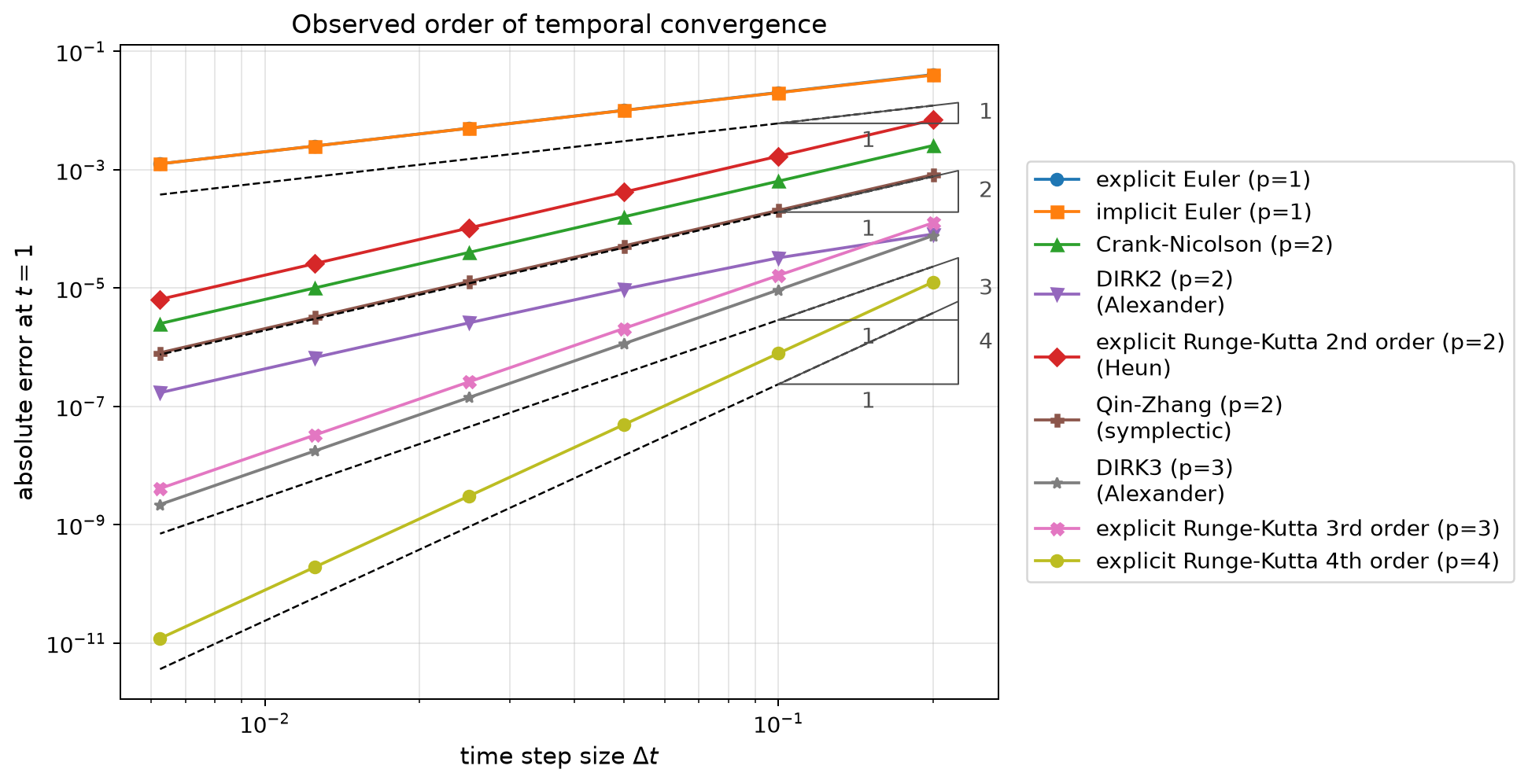
Each curve shows the absolute error \(|u_{\Delta t}(1) - u_{\text{exact}}(1)|\) versus \(\Delta t\) on a log-log scale for \(\dot u = -u + e^t,\ u(0)=0\) (exact solution \(u(t)=\sinh(t)\)); the triangles annotate reference slopes \(\mathcal{O}(\Delta t^p)\) for \(p=1,\ldots,4\) (rise \(p\) over run \(1\)). All schemes attain their expected asymptotic order, or better.

Note: for the simpler equation \(\dot u = e^t\) used in the single-step checks above, the right-hand side is independent of \(u\), so each scheme reduces to a quadrature rule for \(\int e^t\,dt\): Crank-Nicolson and Heun both reduce to the trapezoidal rule and are therefore identical, and the nodes and weights of the explicit RK3 scheme coincide with Simpson's rule (as do RK4's), so both converge with fourth order for that equation. The convergence-sweep equation \(\dot u=-u+e^t\) above avoids this degeneracy, since its right-hand side depends on \(u\).

Benchmark: Linear stability regions

Scheme	negative real-axis cutoff
Explicit Euler	2.0
Heun (RK2)	2.0
Explicit RK3	2.5127
Explicit RK4	2.7853

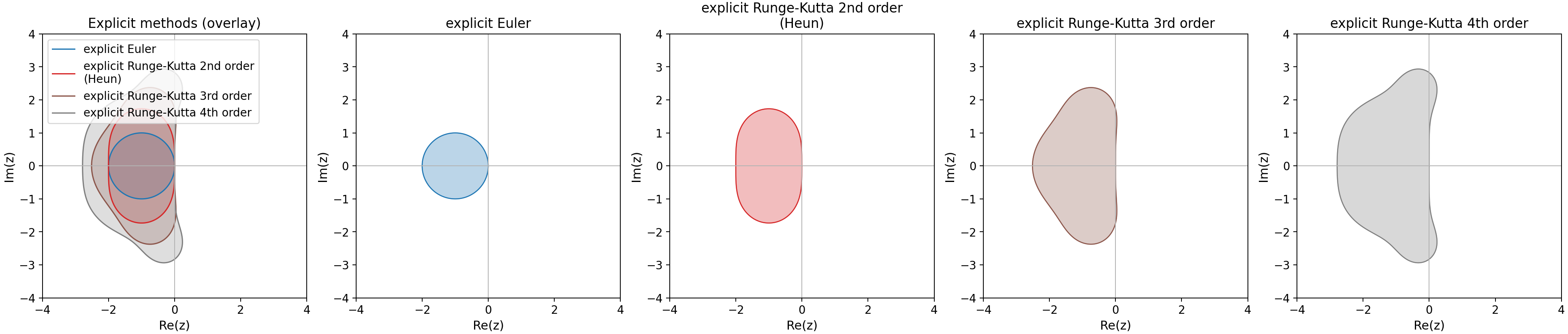
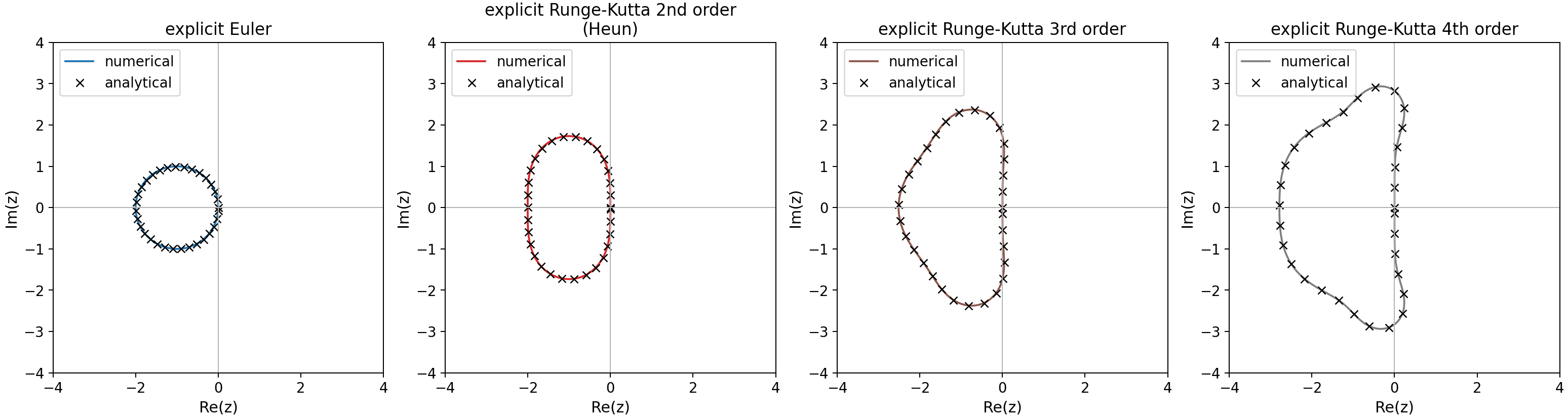
Stability regions of explicit schemes

Numerical vs. analytical stability boundaries

The comparison plot overlays the numerically traced boundary (solid line) with the analytical truncated-exponential boundary \(R(z)=\sum_{k=0}^p z^k/k!\) (crosses); the two coincide to within the Newton tolerance.

Stability regions of implicit schemes

For the implicit schemes, implicit Euler, DIRK2, and DIRK3 are L-stable (the stable region extends unboundedly into the left half-plane, with \(R(z)\to0\)), while Crank-Nicolson and the symplectic Qin-Zhang scheme are A-stable but not L-stable ( \(|R(z)|\to1\) as \(\mathrm{Re}(z)\to-\infty\)). For Qin-Zhang the stability function is \(R(z)=\big((4+z)/(4-z)\big)^2\), so \(|R(iy)|=1\) on the imaginary axis: it introduces no artificial damping, which is the flip side of its symplecticity.

Benchmark: symplecticity

A Runge-Kutta method with weights \(b_i\) and coefficients \(a_{ij}\) is symplectic if and only if it satisfies the condition

\begin{align}b_i a_{ij} + b_j a_{ji} - b_i b_j = 0 \qquad \forall\, i,j, \end{align}

which is exactly the condition under which the method conserves every quadratic first integral exactly. test_timestepmethods_symplectic.cc verifies this condition algebraically for the Qin-Zhang tableau (extracted directly from its Shu-Osher coefficients) and then demonstrates its two consequences on the harmonic oscillator \(\dot q = p,\ \dot p = -q\) (a linear Hamiltonian system with quadratic energy \(H=(q^2+p^2)/2\)):

Phase-space area preservation: the determinant of the one-step propagation matrix is \(1\) to machine precision for Qin-Zhang, whereas it is \(<1\) for implicit Euler and DIRK2 (they contract phase space).
Energy conservation: integrated over 200 periods, Qin-Zhang conserves \(H\) to a relative drift below \(10^{-10}\), while implicit Euler (1st order) damps it away almost entirely and the same second-order DIRK2 also dissipates it — showing that it is symplecticity, not the order of accuracy, that conserves energy.

Symplecticity of the Qin-Zhang scheme

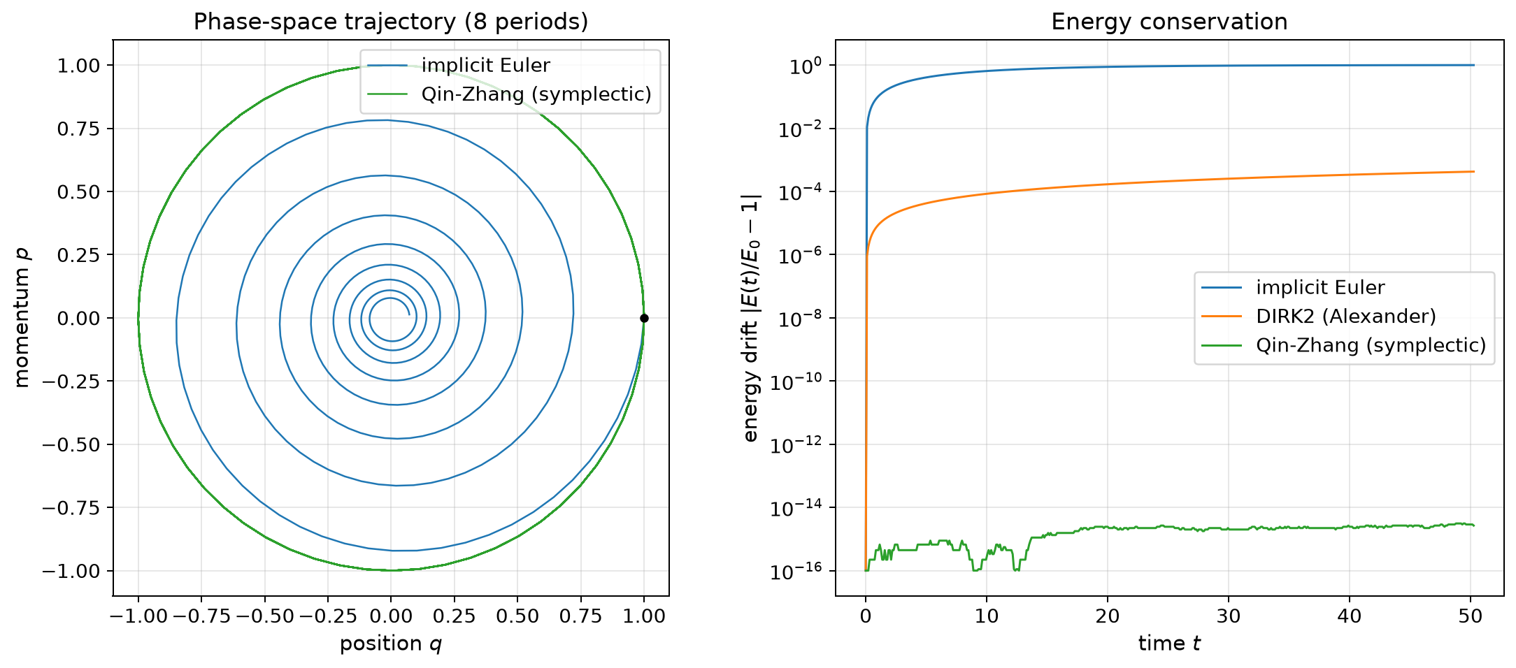
The left panel shows the phase-space trajectory of the symplectic Qin-Zhang scheme (a closed circle) against dissipative implicit Euler (spiralling inward); DIRK2 is omitted from this panel because it is so weakly dissipative that it is visually indistinguishable from the symplectic orbit at this resolution. The right panel shows the energy drift \(|E(t)/E_0-1|\) over time on a logarithmic axis, where that small dissipation becomes visible: Qin-Zhang stays at the machine-precision floor ( \(\sim 10^{-15}\)), whereas implicit Euler loses essentially all the energy and the same second-order DIRK2 drifts by \(\sim 10^{-4}\) — roughly eleven orders of magnitude more than the symplectic scheme, confirming that it is the symplecticity, not the order of accuracy, that conserves the energy.

Reproducing the figures

After building the test_timestepmethods, test_timestepmethods_stabilityregions and test_timestepmethods_symplectic executables, run:

python3 run_benchmarks.py <path-to-build-dir>

This runs all three executables to (re-)generate the JSON data and produces the five figures above via plot_timestepmethods_convergence.py, plot_timestepmethods_stabilityregions.py and plot_timestepmethods_symplectic.py. If run from within <build-dir>/test/experimental/timestepping, the build directory argument can be omitted. Pass --copy-to-doc to additionally copy the figures into doc/doxygen/images/ (used to update the images shown on this page).

🛠 Edit above doc on GitLab