 |
version 3.11-dev
|
|
version 3.11-dev
|
Problem Description
A straight channel of length \(L\) and width \(W\) has a bed that descends along the channel with the slope \(S\). A steady flow of uniform depth \(h_0\) runs down the channel, so the free surface has the slope of the bed. The water depth \(h\) and the depth-averaged velocity components \(u\) along and \(v\) across the channel satisfy the shallow water equations with the bed slope source term and a friction term. The benchmark has two variants, which differ in the friction that balances gravity.
Friction at the side walls. The momentum balance contains the horizontal viscous flux \(\nabla \cdot (\nu_t h \nabla u)\) with a constant eddy viscosity \(\nu_t\), and the velocity vanishes at the side walls \(y = \pm W/2\). For \(h = h_0\), \(v = 0\) and \(u = u(y)\), the momentum balance along the channel reduces to \(0 = g h_0 S + \nu_t h_0 \, \mathrm{d}^2 u / \mathrm{d} y^2\), where \(g\) is the gravitational acceleration. Its solution is the parabolic profile
\begin{align}u(y) = \frac{g S}{8 \nu_t} \left( W^2 - 4 y^2 \right). \end{align}
Friction at the bed. A laminar film flows down an inclined plane, with no slip at the bed and no shear stress at the free surface. Its velocity profile over the depth is a half parabola with the mean velocity \(u\), and the bed shear stress is \(\tau_b = 3 \mu u / h\) (Dumux::FrictionLawViscousNoSlip), where \(\mu\) is the dynamic viscosity and \(\rho\) the density of water. The side walls are free of friction, and the depth-averaged momentum balance reduces to \(0 = g h_0 S - \tau_b / \rho\), with the solution
\begin{align}u = \frac{\rho g S h_0^2}{3 \mu}, \qquad v = 0, \end{align}
which is uniform in the channel.
Parameters
| Parameter | Symbol | Side walls | Bed | Unit |
|---|---|---|---|---|
| Channel length | \(L\) | \(400\) | \(1\) | m |
| Channel width | \(W\) | \(100\) | \(0.1\) | m |
| Bed slope | \(S\) | \(5 \cdot 10^{-5}\) | \(5 \cdot 10^{-6}\) | - |
| Water depth | \(h_0\) | \(10\) | \(10^{-3}\) | m |
| Eddy viscosity | \(\nu_t\) | \(0.1\) | - | m2/s |
| Dynamic viscosity | \(\mu\) | - | \(10^{-3}\) | Pa s |
| Density | \(\rho\) | - | \(1000\) | kg/m3 |
| Gravitational acceleration | \(g\) | \(9.81\) | \(9.81\) | m/s2 |
The maximum velocity of the flow with friction at the side walls is \(u(0) = 6.131\) m/s. The mean velocity of the film is \(u = 1.635 \cdot 10^{-5}\) m/s.
Setup
The shallow water model with the viscous flux (ShallowWater.EnableViscousFlux) is discretized with cell-centered finite volumes (Two-point flux approximation (Tpfa)). The flux over a face is the flux of the exact solution of the Riemann problem with hydrostatic reconstruction of the bed [12], plus a viscous flux computed from the velocity difference between the adjacent cell centers. The bed elevation is constant in each cell. Since the outside state at a boundary face has the bed of the inside cell, a depth prescribed at a boundary face is shifted by the bed difference between face and cell center, such that the free surface elevation at the face is matched.
Friction at the side walls (this folder, grid of \(20 \times 20\) cells in params.input): the discharge per unit width of the exact solution, \(h_0 u(y)\), is prescribed at the inflow and the depth \(h_0\) at the outflow. At the side walls, the viscous flux is computed from the velocity difference between the cell center and the wall (Problem.AlphaWall = 1, no slip). The simulation starts from the exact solution and uses the implicit Euler method up to \(t = 2880\) s, when the flow is steady: on the grid of params.input, the errors at \(t = 2880\) s and \(t = 10^6\) s agree in all printed digits. The tests test_shallowwater_poiseuilleflow (and _parallel, _unstructured on a triangular grid, _unstructured_parallel) compare the solution with a reference solution.
Friction at the bed (folder vertical, grid of \(20 \times 2\) cells): the depth \(h_0\) is prescribed at inflow and outflow, and the side walls are free of friction. The bed shear stress enters the momentum balance as a source term. The stationary problem is solved directly, starting from the exact solution. The test test_shallowwater_poiseuilleflow_vertical compares the solution with a reference solution.
Results
The figure and the tables are produced by running
in the build directory test/freeflow/shallowwater/poiseuilleflow (requires NumPy and Matplotlib). The errors are the relative discrete \(L^2\) errors of the velocity, \(\| e \|_2 / \| u \|_2\) with \(\| e \|_2 = \left( \sum_i |V_i| \, e_i^2 \right)^{1/2}\), where \(e_i\) is the difference to the exact velocity at the center of the cell \(V_i\) with area \(|V_i|\), and \(\| u \|_2\) the norm of the exact velocity evaluated in the same way. The flow with friction at the side walls is computed up to \(t = 10^6\) s with time steps of up to \(10^5\) s.
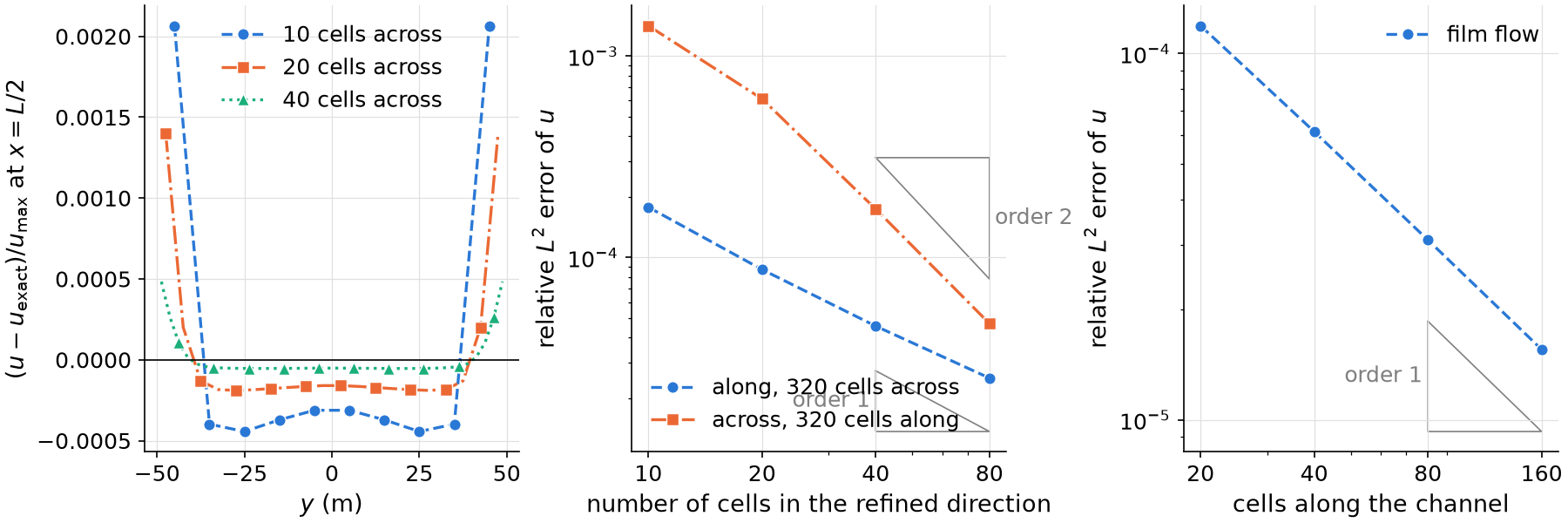
Friction at the side walls. The grid is refined along the channel with 320 cells across, and across the channel with 320 cells along.
| grid (along × across) | rel. \(L^2\) error \(u\) | rate |
|---|---|---|
| 10 × 320 | 1.776e-04 | - |
| 20 × 320 | 8.714e-05 | 1.03 |
| 40 × 320 | 4.567e-05 | 0.93 |
| 80 × 320 | 2.523e-05 | 0.86 |
| grid (along × across) | rel. \(L^2\) error \(u\) | rate |
|---|---|---|
| 320 × 10 | 1.411e-03 | - |
| 320 × 20 | 6.120e-04 | 1.21 |
| 320 × 40 | 1.738e-04 | 1.82 |
| 320 × 80 | 4.704e-05 | 1.89 |
Across the channel, the error converges with approximately second order, the order of the two-point viscous flux. The largest errors are in the cells next to the walls. Along the channel, the exact solution does not vary, and the error converges with approximately first order. In the steady state, the mass flux over each face equals the discharge prescribed at the inflow. The bed is constant in each cell, so the hydrostatic reconstruction compares the depths \(h\) and \(h - S \Delta x\) at a face, where \(\Delta x\) is the cell size along the channel. For these states, the mass flux of the exact Riemann solver exceeds \(h u\) by \((c - u) S \Delta x / 2\), to first order in \(S \Delta x\), with the celerity \(c = \sqrt{g h_0}\). The velocity in the cells is therefore smaller than the exact one by \((c - u) S \Delta x / (2 h_0)\). The script compares the mean of this estimate over the width with the mean velocity error in the middle of the channel:
| grid (along × across) | mean velocity error (m/s) | \(-(c - u) S \Delta x / (2 h_0)\), mean over the width (m/s) |
|---|---|---|
| 10 × 320 | -5.854e-04 | -5.817e-04 |
| 20 × 320 | -2.926e-04 | -2.909e-04 |
| 40 × 320 | -1.465e-04 | -1.454e-04 |
| 80 × 320 | -7.339e-05 | -7.271e-05 |
The rates along the channel decrease under refinement as the error approaches that of the 320 cells across.
Friction at the bed. The grid is refined along the channel.
| grid (along × across) | rel. \(L^2\) error \(u\) | rate |
|---|---|---|
| 20 × 2 | 1.191e-04 | - |
| 40 × 2 | 6.119e-05 | 0.96 |
| 80 × 2 | 3.097e-05 | 0.98 |
| 160 × 2 | 1.556e-05 | 0.99 |
The error converges with approximately first order. Here, the depth is prescribed at both ends and the discharge results from the momentum balance. On 20 cells, the relative error of the velocity is \(1.19 \cdot 10^{-4}\), close to \(S \Delta x / (2 h_0) = 1.25 \cdot 10^{-4}\), the step of the bed at a face relative to twice the depth. The script repeats the 20-cell run with the slope \(10 S\) and with the depth \(2 h_0\); the relative errors are \(1.19 \cdot 10^{-3}\) and \(6.04 \cdot 10^{-5}\), again 0.95 to 0.97 times \(S \Delta x / (2 h_0)\).
The test test_shallowwater_poiseuilleflow_convergence refines the grid along the channel ( \(10, 20, 40\) cells, 160 cells across) and across the channel ( \(20, 40, 80\) cells, 160 cells along) and checks that the mean convergence rates of the relative \(L^2\) error are at least 0.85 and 1.6. The test test_shallowwater_poiseuilleflow_vertical_convergence runs the film flow on \(20, 40, 80\) cells and checks that the mean rate is at least 0.9.
3.11-dev
Generated by  1.16.1