 |
version 3.11-dev
|
|
version 3.11-dev
|
Problem Description
Both benchmarks simulate unsaturated water flow in a 1D soil column using the Richards equation. They were originally proposed by Vanderborght et al. (2005) [101] and are part of the collaborative benchmark project for root–soil interaction models (Schnepf et al. 2020 [88]) in which DuMux participated as a reference simulator.
The governing equation is the Richards equation for the volumetric water content \(\theta\) [-]:
\begin{align}\frac{\partial \theta}{\partial t} = \frac{\partial}{\partial z}\left[K(\theta)\left(\frac{\partial h}{\partial z} - 1\right)\right]\end{align}
where \(h\) [cm] is the pressure head (negative for unsaturated conditions), \(K(\theta)\) [cm day \(^{-1}\)] is the unsaturated hydraulic conductivity, and \(z\) [cm] is the vertical coordinate (positive upward). The water retention and conductivity curves follow the van Genuchten–Mualem model:
\begin{align}\theta(h) = \theta_r + (\theta_s - \theta_r)\left[1 + |\alpha h|^n\right]^{-m}, \quad m = 1 - \tfrac{1}{n}\end{align}
\begin{align}K(\theta) = K_\mathrm{sat}\, S_e^{1/2}\left[1 - \left(1 - S_e^{1/m}\right)^m\right]^2, \quad S_e = \frac{\theta - \theta_r}{\theta_s - \theta_r}\end{align}
Three soil types (sand, loam, clay) are tested in each scenario.
Benchmark M2.1 — Infiltration
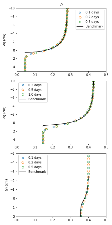
A 1D soil column of depth 200 cm with uniform initial pressure head \(h_i = -400\) cm is subjected to a large infiltration flux of \(J = -1000\) mm day \(^{-1}\) at the top surface (negative convention: influx). The top boundary switches to a Dirichlet condition ( \(h = 0\) cm) once the imposed flux would require super-saturation. The bottom boundary imposes free drainage (gravity-driven outflow only). Gravity is enabled ( \(g = 9.81\) m s \(^{-2}\)).
| Soil | Simulation times |
|---|---|
| Sand | 0.1, 0.2, 0.3 days |
| Loam | 0.2, 0.5, 1.0 days |
| Clay | 0.1, 0.2, 0.5 days |
Benchmark M2.2 — Evaporation
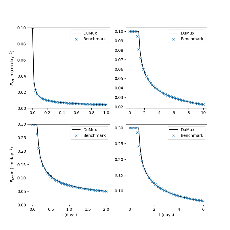
A 1D soil column of depth 100 cm is subjected to a potential evaporation flux at the top. The top boundary switches to a Dirichlet condition ( \(h = -10{,}000\) cm) once the soil can no longer sustain the potential rate. The bottom boundary is no-flux. Gravity is neglected (consistent with the analytical reference solution).
| Soil | Initial head | Potential evaporation | Duration |
|---|---|---|---|
| Sand | \(h_i = -40\) cm | 1.0 mm day \(^{-1}\) | 1 day |
| Loam (low rate) | \(h_i = -200\) cm | 1.0 mm day \(^{-1}\) | 10 days |
| Loam (high rate) | \(h_i = -200\) cm | 3.0 mm day \(^{-1}\) | 2 days |
| Clay | \(h_i = -200\) cm | 3.0 mm day \(^{-1}\) | 6 days |
Parameters
Van Genuchten soil parameters (Schnepf et al. 2020, Table 3):
| Parameter | Symbol | Sand | Loam | Clay | Unit |
|---|---|---|---|---|---|
| Residual water content | \(\theta_r\) | 0.045 | 0.08 | 0.10 | - |
| Saturated water content | \(\theta_s\) | 0.43 | 0.43 | 0.40 | - |
| Van Genuchten \(\alpha\) | \(\alpha\) | 0.15 | 0.04 | 0.01 | cm \(^{-1}\) |
| Van Genuchten \(n\) | \(n\) | 3.0 | 1.6 | 1.1 | - |
| Mualem exponent | \(\ell\) | 0.5 | 0.5 | 0.5 | - |
| Saturated hydraulic conductivity | \(K_\mathrm{sat}\) | 1000 | 50 | 10 | cm day \(^{-1}\) |
Analytical Solution — M2.1 Infiltration (Travelling Wave)
The analytical solution (Vanderborght 2005, Eq. 56–60; Schnepf 2020, Eq. 4) assumes the infiltration front travels as a wave of constant shape. Introducing the transformed coordinate:
\begin{align}\eta(x, t) = |x| - \frac{K_\mathrm{sur} - K_i}{\theta_\mathrm{sur} - \theta_i}\, t\end{align}
where \(K_\mathrm{sur} = K(\theta_\mathrm{sur})\) and \(K_i = K(\theta_i)\) are the hydraulic conductivities at the surface and initial water contents respectively, the relative position \(\Delta\eta(\theta) = \eta - \eta_a\) (with \(\theta_a = (\theta_\mathrm{sur} + \theta_i)/2\)) satisfies the implicit relation:
\begin{align}\Delta\eta(\theta) = (\theta_\mathrm{sur} - \theta_i)\int_\theta^{\theta_a} \frac{D(\theta')}{(K_\mathrm{sur} - K_i)(\theta' - \theta_i) - (K(\theta') - K_i)(\theta_\mathrm{sur} - \theta_i)}\,\mathrm{d}\theta'\end{align}
where \(D(\theta) = K(\theta)\,\mathrm{d}h/\mathrm{d}\theta\) [cm \(^2\) day \(^{-1}\)] is the hydraulic diffusivity. This integral is evaluated numerically and inverted by table lookup to recover \(\theta(\Delta\eta)\). The solution assumes boundaries at \(z = \pm\infty\) and is valid when the front is far from the actual boundaries.
Analytical Solution — M2.2 Evaporation (Desorptivity)
The analytical solution (Vanderborght 2005, Eq. 39–47; Lockington 1994) is based on the desorptivity \(S_w\) [cm day \(^{-1/2}\)], which is computed from the diffusivity integral via:
\begin{align}S_w = (\theta_i - \theta_s^*)\sqrt{\frac{4}{\mu}\int_0^1 D(\Theta)\,\mathrm{d}\Theta}\end{align}
where \(\Theta = (\theta - \theta_s^*)/(\theta_i - \theta_s^*)\) is the effective water content, \(\theta_s^*\) is the surface water content at the critical pressure head, and \(\mu\) is a shape factor (Vanderborght 2005, Eq. 41). The actual evaporation rate \(E_\mathrm{act}\) [mm day \(^{-1}\)] is:
\begin{align}E_\mathrm{act}(t) = \begin{cases} E_\mathrm{pot} & t < t_\mathrm{pot} \\[4pt] \dfrac{S_w}{2\sqrt{t' + t - t_\mathrm{pot}}} & t \geq t_\mathrm{pot} \end{cases}\end{align}
where \(t_\mathrm{pot} = S_w^2 / (2\,E_\mathrm{pot}^2)\) is the critical time at which the actual rate first falls below the potential rate, and \(t' = t_\mathrm{pot}/2\). This is an approximate solution valid for gravity-free, semi-infinite domains with less than 1% error (Lockington 1994).
Setup
The domain is discretized as a 1D interval using a Dune::YaspGrid with TensorProductCoordinates. For the infiltration scenario (M2.1), a uniform grid of 300 cells spanning [−2 m, 0 m] is used. For the evaporation scenario (M2.2), a graded grid of 1000 cells spanning [−1 m, 0 m] with refinement towards the top surface (grading factor −0.99) resolves the near-surface drying front. The Richards with Two-point flux approximation (Tpfa) is used in both cases. Time integration uses an adaptive implicit time loop with a specialized RichardsNewtonSolver and analytic Jacobian. The van Genuchten fluid–matrix interaction is provided by Dumux::FluidMatrix::VanGenuchten.
Results
To reproduce the infiltration results (M2.1) and produce the comparison plot, run:
To reproduce the evaporation results (M2.2), run:
The infiltration script produces benchmark_infiltration.png: water content \(\theta\) versus the transformed coordinate \(\Delta\eta\) [cm] for all three soil types at the specified output times. Numerical results (markers) are compared against the analytical travelling-wave solution (solid line). This reproduces the right column of Fig. 4 in Vanderborght et al. (2005).
The evaporation script produces benchmark_evaporation.png: actual evaporation rate \(E_\mathrm{act}\) [cm day \(^{-1}\)] versus time [days] for all four evaporation scenarios. Numerical results (solid line) are compared against the desorptivity-based analytical reference (markers). This reproduces Fig. 5 of Vanderborght et al. (2005).
 3.11-dev
Generated by
3.11-dev
Generated by  1.16.1