 |
version 3.11-dev
|
|
version 3.11-dev
|
Problem Description
A fluid-saturated poroelastic slab \([-a, a] \times [-b, b]\) in plane strain is squeezed between two rigid, frictionless and impermeable plates [62]. At \(t = 0\), a force \(2F\) per unit length is applied to each plate. The lateral sides \(x = \pm a\) are traction-free and drained. The load is first carried by the pore fluid: the instantaneous (undrained) response raises the pore pressure uniformly to \(p^+\). The fluid then drains through the lateral sides. Because the drained outer part of the slab softens, load is transferred to the center, where the pore pressure first rises above \(p^+\) before it decays (Mandel-Cryer effect). By symmetry, only the quarter \([0, a] \times [0, b]\) (shaded) is simulated.
The displacement \(\mathbf{u}\) and the pore pressure \(p\) satisfy the momentum balance and the fluid mass balance
\begin{align}\nabla \cdot \left( \boldsymbol{\sigma}' - \alpha p \mathbf{I} \right) = \mathbf{0}, \qquad \boldsymbol{\sigma}' = 2 G \boldsymbol{\varepsilon} + \lambda \, \mathrm{tr}(\boldsymbol{\varepsilon}) \mathbf{I}, \qquad \boldsymbol{\varepsilon} = \tfrac{1}{2}\left( \nabla \mathbf{u} + \nabla \mathbf{u}^T \right),\end{align}
\begin{align}\frac{\partial \zeta}{\partial t} - \nabla \cdot \left( \frac{k}{\mu} \nabla p \right) = 0, \qquad \zeta = \phi + \phi_0 \frac{p - p^+}{K_f},\end{align}
where \(\boldsymbol{\sigma}'\) is the effective stress, \(G\) and \(\lambda\) are the drained Lamé parameters, \(\alpha\) is the Biot coefficient, \(k\) is the permeability, \(\mu\) is the fluid viscosity and \(K_f\) is the bulk modulus of the fluid. The fluid content \(\zeta\) per unit volume of the undeformed slab is the porosity \(\phi\) plus the compression of the pore fluid. The porosity is the pore volume per unit volume of the undeformed slab [28],
\begin{align}\phi = \phi_0 + \alpha \left( \varepsilon_v - \varepsilon_{v,0} \right) + \frac{p - p^+}{N}, \qquad \frac{1}{N} = \frac{(\alpha - \phi_0)(1 - \alpha)}{K},\end{align}
with the volumetric strain \(\varepsilon_v = \nabla \cdot \mathbf{u}\), the drained bulk modulus \(K\), and the porosity \(\phi_0\) and volumetric strain \(\varepsilon_{v,0}\) of the undrained state at \(t = 0\). For \(\alpha < 1\), the term with \(N\) accounts for the compressibility of the solid grains with bulk modulus \(K_s = K/(1-\alpha)\). The fluid content is that of Biot's theory, \(\zeta - \phi_0 = \alpha (\varepsilon_v - \varepsilon_{v,0}) + (p - p^+)/M\), with the Biot modulus \(1/M = \phi_0/K_f + 1/N\). The single-phase model solves this linear mass balance with a constant fluid density and \(\zeta\) in place of the porosity in the storage term. A pressure-dependent density \(\varrho_0(1 + p/K_f)\) instead would add terms of relative size \(p/K_f\), up to \(8 \times 10^{-4}\) here, which are not part of the analytical solution: with such a density, the convergence rate of the pressure error in the test below drops from 1.75 (grids \(40 \times 4\) to \(80 \times 8\)) to 0.50 (grids \(160 \times 16\) to \(320 \times 32\)).
Boundary conditions on the quarter domain:
| Boundary | Mechanics | Flow |
|---|---|---|
| \(x = 0\) (symmetry) | \(u_x = 0\), zero shear traction | no flow |
| \(y = 0\) (symmetry) | \(u_y = 0\), zero shear traction | no flow |
| \(y = b\) (rigid plate) | \(u_y\) of the analytical solution, zero shear traction | no flow |
| \(x = a\) | traction-free | \(p = 0\) |
The rigid plate is represented by its displacement, which is uniform along the plate and follows from the analytical solution. Initial conditions are the undrained response at \(t = 0\),
\begin{align}p = p^+ = \frac{F B (1+\nu_u)}{3a}, \qquad u_x = \frac{F \nu_u}{2 G a} x, \qquad u_y = -\frac{F (1-\nu_u)}{2 G a} y,\end{align}
with the Skempton coefficient \(B = \alpha M / K_u\), the undrained bulk modulus \(K_u = K + \alpha^2 M\) and the undrained Poisson's ratio \(\nu_u = (3K_u - 2G)/(2(3K_u + G))\).
Analytical Solution
\begin{align}p = 2 p^+ \sum_{n=1}^{\infty} \frac{\sin\beta_n}{\beta_n - \sin\beta_n\cos\beta_n} \left( \cos\frac{\beta_n x}{a} - \cos\beta_n \right) e^{-\beta_n^2 c t / a^2},\end{align}
\begin{align}u_x = \left( \frac{\nu}{2} - \nu_u \sum_{n=1}^{\infty} S_n \right) \frac{F x}{G a} + \frac{F}{G} \sum_{n=1}^{\infty} \frac{\cos\beta_n}{\beta_n - \sin\beta_n\cos\beta_n} \sin\frac{\beta_n x}{a} \, e^{-\beta_n^2 c t / a^2},\end{align}
\begin{align}u_y = \left( -\frac{1-\nu}{2} + (1-\nu_u) \sum_{n=1}^{\infty} S_n \right) \frac{F y}{G a}, \qquad S_n = \frac{\sin\beta_n\cos\beta_n}{\beta_n - \sin\beta_n\cos\beta_n} e^{-\beta_n^2 c t / a^2},\end{align}
where \(\nu\) is the drained Poisson's ratio, \(\beta_n\) is the \(n\)-th positive root of \(\tan\beta / \beta = (1-\nu)/(\nu_u-\nu)\), and
\begin{align}c = \frac{k}{\mu} M \frac{K + \frac{4}{3} G}{K_u + \frac{4}{3} G}\end{align}
is the consolidation coefficient. The implementation evaluates the first \(N_\beta\) terms of each series (Problem.NumSeriesTerms).
Parameters
| Parameter | Symbol | Value | Unit |
|---|---|---|---|
| Force per unit length on each plate | \(2F\) | \(1.2 \times 10^{9}\) | N/m |
| Half-width, half-height | \(a\), \(b\) | 100, 10 | m |
| Drained Young's modulus | \(E\) | \(5.94 \times 10^{9}\) | Pa |
| Drained Poisson's ratio | \(\nu\) | 0.2 | - |
| Biot coefficient | \(\alpha\) | 1.0 | - |
| Porosity at \(t = 0\) | \(\phi_0\) | 0.2 | - |
| Fluid bulk modulus | \(K_f\) | \(3.3 \times 10^{9}\) | Pa |
| Fluid density | \(\varrho\) | 1000 | kg/m³ |
| Fluid viscosity | \(\mu\) | \(10^{-3}\) | Pa s |
| Permeability | \(k\) | \(9.87 \times 10^{-14}\) | m² |
| Number of series terms | \(N_\beta\) | 240 | - |
The derived parameters are \(G = 2.475\) GPa, \(K = 3.3\) GPa, \(M = 16.5\) GPa, \(K_u = 19.8\) GPa, \(B = 0.833\), \(\nu_u = 0.44\), \(c = 0.465\) m²/s, \(a^2/c = 21\,493\) s and \(p^+ = 2.4\) MPa. The test test_md_mandel_compressible_grains uses \(\alpha = 0.7\) and \(K_f = 2.2\) GPa instead, which gives \(K_s = 11\) GPa, \(M = 7.33\) GPa, \(B = 0.745\), \(\nu_u = 0.340\) and \(p^+ = 2.0\) MPa.
Setup
The quarter domain is discretized with a structured grid of \(40 \times 4\) cells. The flow problem (1p) uses the cell-centered two-point flux approximation (Two-point flux approximation (Tpfa)), the poroelastic problem (Solid mechanics with fluid pressure) uses the Box scheme (PQ1 CVFE (Box) scheme) on the same grid. The two problems are coupled through the pressure in the effective stress and the porosity in the storage term, and solved monolithically (Multidomain framework) with Newton's method and a direct linear solver. The time integration uses the multi-stage assembler in dumux/experimental; implicit Euler (default), Crank-Nicolson and a three-stage, third-order diagonally implicit Runge-Kutta method are selected with TimeLoop.Scheme. The time step size starts at TimeLoop.Dt and is adapted to the number of Newton iterations up to TimeLoop.MaxTimeStepSize; the solution is written at the times TimeLoop.CheckPoints.
Results
The plots below are produced by running
in the build directory test/multidomain/poromechanics/mandel. The script runs the simulation until \(t = 20\,000\) s and compares the pressure in the cells and the horizontal displacement of the plate with the analytical solution. The pressure at the center first rises to \(1.081\,p^+\) at \(t \approx 1400\) s (Mandel-Cryer effect) and then decays. The images of this page are regenerated by passing doc/doxygen/images of the DuMux source directory as second argument.
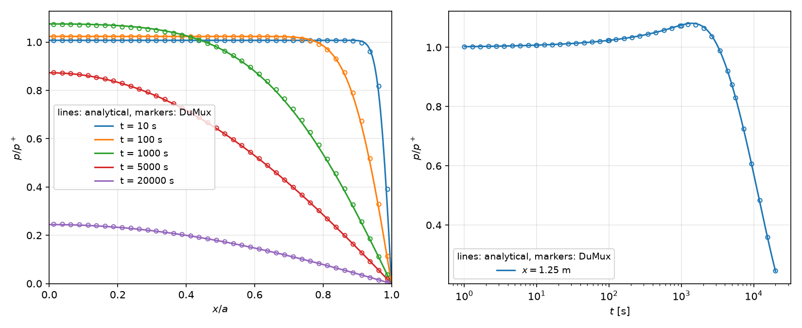
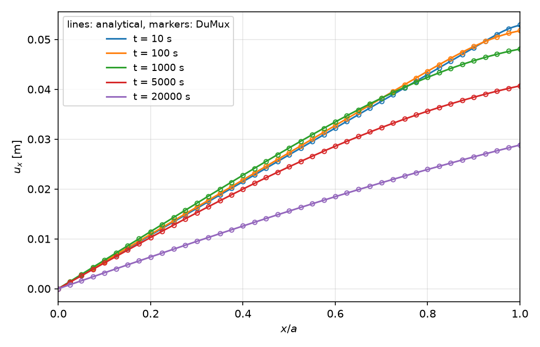
With the parameters above (implicit Euler, time step size growing from 0.1 s to at most 10 s), the relative discrete \(L^2\) error of the pressure at \(t = 5000\) s is \(3.5 \times 10^{-4}\) for \(\alpha = 1\) and \(4.1 \times 10^{-4}\) for \(\alpha = 0.7\).
The test test_md_mandel_convergence (script convergencetest.py) refines the grid twice and checks that the discrete \(L^2\) errors of \(p\) and \(u_x\) at \(t = 1000\) s decrease with a rate of at least 1.9. It uses the third-order DIRK scheme so that the time discretization error is smaller than the spatial error. On the grids \(40 \times 4\) to \(320 \times 32\), the errors are
| Grid | \(\lVert p - p_\mathrm{exact} \rVert_{L^2}\) [Pa m] | rate | \(\lVert u_x - u_{x,\mathrm{exact}} \rVert_{L^2}\) [m²] | rate |
|---|---|---|---|---|
| \(40 \times 4\) | \(1.92 \times 10^{4}\) | - | \(1.15 \times 10^{-4}\) | - |
| \(80 \times 8\) | \(4.79 \times 10^{3}\) | 2.00 | \(2.87 \times 10^{-5}\) | 2.00 |
| \(160 \times 16\) | \(1.20 \times 10^{3}\) | 2.00 | \(7.17 \times 10^{-6}\) | 2.00 |
| \(320 \times 32\) | \(2.97 \times 10^{2}\) | 2.01 | \(1.79 \times 10^{-6}\) | 2.01 |
3.11-dev
Generated by  1.16.1