 |
version 3.11-dev
|
|
version 3.11-dev
|
Problem Description
CO2 is injected at the constant volumetric rate \(Q\) through a vertical well of radius \(r_w\) into a horizontal, homogeneous aquifer of height \(H\) that is initially filled with brine. The well is open over the entire height, the top and the bottom of the aquifer are impermeable, and the pressure is fixed at the outer radius \(R\). The injected CO2 is less dense and less viscous than the brine, so it forms a plume of thickness \(h(r, t)\) that overrides the brine below the top of the aquifer and extends to the radius \(r_p(t)\). The setup and the parameters are those of the injection example of Nordbotten and Celia (2006) [78].
At the well, the mass fluxes of CO2 and brine into the aquifer are \(q_n = \varrho_n Q / (2 \pi r_w H)\) and \(q_w = 0\), where \(\varrho_n\) is the density of CO2. At the outer radius, the brine pressure at the bottom of the aquifer is \(P_w = 3.15 \cdot 10^{7}\) Pa and the aquifer contains no CO2, \(\bar S_n = 0\). The top and the bottom of the aquifer are impermeable, and gravity acts in the negative \(z\) direction.
The flow is simulated with the two-phase vertical-equilibrium model (2pve). On a one-dimensional radial coarse grid, each cell of which represents a vertical column, the mass balance of each phase \(\alpha \in \{w, n\}\) reads
\begin{align}\frac{\partial (\bar\phi \varrho_\alpha \bar S_\alpha)}{\partial t} - \nabla_h \cdot \left\{ \varrho_\alpha \bar\lambda_\alpha \bar K \nabla_h P_\alpha \right\} = 0,\end{align}
where \(\nabla_h\) is the horizontal gradient, \(\bar\phi\) and \(\bar K\) are the vertically averaged porosity and permeability, \(\bar S_\alpha\) is the vertically averaged saturation, \(\bar\lambda_\alpha\) the vertically averaged mobility and \(P_\alpha\) the pressure at the bottom of the column. The injected CO2 is the phase \(n\) and the brine the phase \(w\). The vertical distribution of the saturations in each column is reconstructed from the Brooks-Corey capillary pressure in hydrostatic equilibrium. The entry pressure \(p_e\) is chosen such that the capillary fringe of height \(p_e / ((\varrho_w - \varrho_n) g)\), with the gravitational acceleration \(g\), is small compared to \(H\), so that the reconstructed interface between the phases approximates the sharp interface of the similarity solution.
The simulated gas plume distance is the effective gas plume distance
\begin{align}z_{p,\mathrm{eff}} = H \left( 1 - \frac{\bar S_n}{1 - S_{wr}} \right),\end{align}
which corresponds to a plume that contains the injected CO2 at the saturation \(1 - S_{wr}\), where \(S_{wr}\) is the residual brine saturation. This is the definition that [78] use for their numerical reference solutions. It is output as effectiveGasPlumeDistance. In the sharp-interface limit, it equals the gas plume distance \(z_p\) of the model, the lower boundary of the mobile CO2, which is output as zp. With a finite capillary fringe, the two differ.
Analytical Solution
For a sharp interface and incompressible fluids, the plume thickness \(h\) depends only on the similarity variable
\begin{align}\chi = \frac{2 \pi H \phi (1 - S_{wr}) r^2}{Q t},\end{align}
where \(r\) is the radial distance from the well and \(t\) the time. If buoyancy is negligible compared to the viscous forces, the dimensionless plume thickness is (eq. (14) in [78])
\begin{align}\frac{h}{H} = \begin{cases} 1 & \chi \leq 2/\lambda, \\ \frac{1}{\lambda - 1} \left( \sqrt{\frac{2 \lambda}{\chi}} - 1 \right) & 2/\lambda < \chi < 2 \lambda, \\ 0 & \chi \geq 2 \lambda, \end{cases}\end{align}
with the mobility ratio \(\lambda = \mu_w / \mu_n\) of the CO2 plume and the brine, where \(\mu_\alpha\) is the dynamic viscosity of phase \(\alpha\). The gas plume distance is \(H - h\). The solution is the limit of vanishing gravity number
\begin{align}\Gamma = \frac{2 \pi (\varrho_w - \varrho_n) g k H^2}{\mu_w Q},\end{align}
where \(k\) is the permeability. The simulation includes buoyancy, so its deviation from the similarity solution decreases with \(\Gamma\).
The deviation is measured by the relative gas plume distance error
\begin{align}e = \frac{1}{H r_p} \int_{r_w}^{R} \left| z_{p,\mathrm{eff}} - (H - h) \right| \mathrm{d}r,\end{align}
the mean deviation of the gas plume distance over the plume extent \(r_p = \sqrt{2 \lambda Q t / (2 \pi H \phi (1 - S_{wr}))}\), relative to \(H\).
Parameters
| Parameter | Symbol | Value | Unit |
|---|---|---|---|
| Aquifer height | \(H\) | 15 | m |
| Permeability | \(k\) | \(1.974 \cdot 10^{-14}\) (20 mD) | m² |
| Porosity | \(\phi\) | 0.15 | - |
| Brine density | \(\varrho_w\) | 1099 | kg/m³ |
| CO2 density | \(\varrho_n\) | 733 | kg/m³ |
| Brine viscosity | \(\mu_w\) | \(5.11 \cdot 10^{-4}\) | Pa s |
| CO2 viscosity | \(\mu_n\) | \(6.1 \cdot 10^{-5}\) | Pa s |
| Injection rate | \(Q\) | \(1.389 \cdot 10^{-3}\) (120 m³/day) | m³/s |
| Injection time | \(t_{end}\) | \(8.64 \cdot 10^{8}\) (10000 days) | s |
| Well radius | \(r_w\) | 0.1 | m |
| Outer radius | \(R\) | 2000 | m |
| Initial brine pressure at the bottom of the aquifer, fixed at \(r = R\) | \(P_w\) | \(3.15 \cdot 10^{7}\) | Pa |
| Residual saturations | \(S_{wr}\), \(S_{nr}\) | 0 | - |
| Brooks-Corey entry pressure | \(p_e\) | 100 | Pa |
| Brooks-Corey parameter | - | 2 | - |
| Mobility ratio | \(\lambda\) | 8.38 | - |
| Gravity number | \(\Gamma\) | 0.141 | - |
The injected volume is \(1.2 \cdot 10^6\) m³ and the capillary fringe is 0.028 m high.
Setup
The domain spans the radial and the vertical coordinate and is rotated about the axis of the well. The coarse grid is one-dimensional with 400 radial cells, extruded by the aquifer height, and the fine grid has 400 × 30 cells. Both fluids are incompressible with constant properties. The equations are discretized with the cell-centered two-point flux approximation (Two-point flux approximation (Tpfa)) and the implicit Euler method with a maximum time step size of 10 days.
The test suite runs two cases and compares the relative gas plume distance error at the end of the simulation to a tolerance:
Results
To run the simulations and produce the figures, run in the build directory of the test:
The script produces three figures:
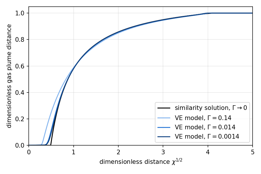
The similarity solution is the limit \(\Gamma \to 0\) for a sharp interface. With 400 radial cells and \(p_e = 100\) Pa, the relative gas plume distance error at the end of the simulation is 0.0201 for \(\Gamma = 0.141\), 0.0051 for \(\Gamma = 0.0141\) and 0.0034 for \(\Gamma = 0.00141\). For \(\Gamma = 0.141\), the deviation is largest close to the well: with buoyancy, the CO2 fills the aquifer down to its bottom only up to \(\chi^{1/2} = 0.28\), the gas plume distance being below \(0.01 H\), compared to \(\chi^{1/2} = (2/\lambda)^{1/2} = 0.49\) in the similarity solution.
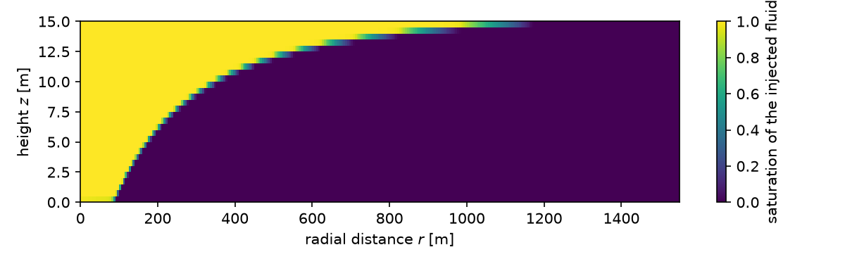
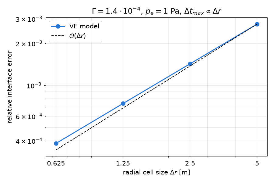
For \(\Gamma = 1.4 \cdot 10^{-4}\) and \(p_e = 1\) Pa, the capillary fringe is \(2.8 \cdot 10^{-4}\) m high. Refining the radial cell size from 5 m to 2.5, 1.25 and 0.625 m together with the maximum time step size from 864 s to 432, 216 and 108 s decreases the relative gas plume distance error from \(2.75 \cdot 10^{-3}\) to \(1.43 \cdot 10^{-3}\), \(7.41 \cdot 10^{-4}\) and \(3.83 \cdot 10^{-4}\). The observed convergence rate is 0.95 for each refinement, close to the first order of the upwind two-point flux approximation and of the implicit Euler method.
The numerical plots in the documentation are regenerated with
3.11-dev
Generated by  1.16.1